The Ising model is one of the most studied model in statistical physics. It was first proposed as a model to explain the orgin of magnetism arising from bulk materials containing many interacting magnetic dipoles and/or spins. In this model, space is divided up into a discrete lattice with a magnetic spin on each site. An Ising spin is permitted to take just two value, +1 (up) or -1 (down). Each spin interacts with its nearest neighbors and
an external magnetic field B through the following Hamiltonian,

where J>0 gives the spin-spin interaction strength and  indicates the sum over all nearest neighbor pairs (i,j) on the lattice. (see the following picture)
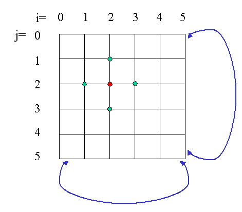
In this 2D square lattice, the red site iteracts only with its four nearest neighbors indicated by the green circles. The lattice shown is a small 5x5 lattice with periodic boundary condition meaning that the leftmost sites are identified with the rightmost ones. Similarly, the top sites are identified with the bottom ones (symbolically indicated by the blue arrows). In general, one is interested in the statistical properties, such as the average total magnetization M or the internal energy U of this network in the limit when the system size is large. The different possible states of the Ising model are characterized by the different sets of spin values {si}. Since each spin can only take on two possible values [+1 (up) or -1 (down)], the total number of states (all combinations of up and down spins) possible for a model with N sites (e.g. a 5x5 2D model will have N=25 sites) is 2N. The Hamiltonian gives the total energy of the lattice with a particular spin configuration. With the sign chosen for J>0, the lowest energy state corresponds to the one with all the spins line up with each other and with the same direction as the magnetic field B (ferromagnetic case). [Note that the J<0 case corresponds to the anti-ferromagnetic case in which the spins will perfer to line up anti-parallel with each other.]
Using the standard machinery in statistical physics, the marcorscopic properties of the system is completely described by the partition function of the model, Note: The weighted averages defined in the previous two equations can be calculated as a simple mean of the relevant quantity f over the number of the Metropolis steps - M, i.e., One of the most dramatic effect for a magnetic system is the sudden emergence of coherence magnetic domains when the temperature of the system is lowered pass a critical value. The 2D Ising model is one of the simplest model that demonstrates this critical transition with Tc>0. Onsager in 1944, by pure analytical perseverance, proved this fact by providing the first exact solution to the 2D Ising model. While exact analytic solutions are important, numerical simultations of magnetic models like the 2D Ising model are also important and they are easily accessible by Monte Carlo methods.
For this problem, you need to do the following:
Hints:

where k is the Boltzman constant and T is the temperature of the system and the sum is over all possible configurations of spins for the system. For example, the expectation value of the total energy

where b=1/kT and the specific heat of the system is given by
 .
.
The exponential factor inside the partition function is called the Boltzman factor and all statistical averages at equilibrium is calculated with respect to this weighting factor. Thus, the average energy of the system

where the sum is over all possible spin configurations and we use X as a label to denote a particular spin configuration of the system. (One can easily see that this expression is equivalent to the one given above.) Another important statistic average relevant to the Ising system is the average magnetization of the system defined by

The internal sum is over all sites for a particular configuration X and the external sum is again over all possible configurations. Often, it is rather the average magnetization per site  that one will often use to characterize the macroscopic state of the system.
 .
.
 and the specific heat c of the system

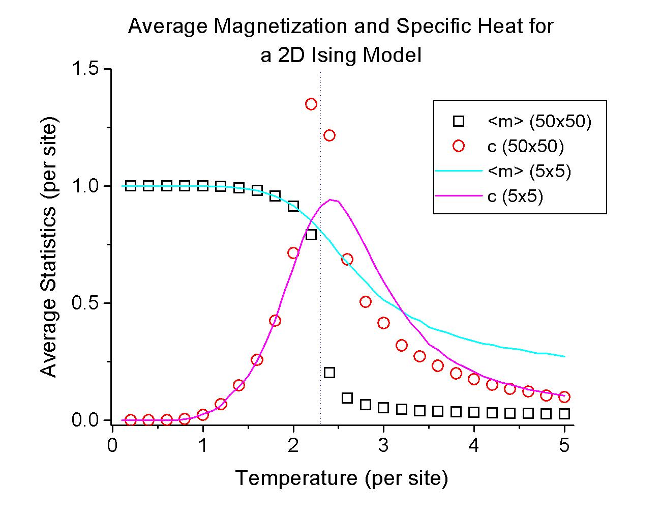
for temperatures from T=5 down to 0 with steps of 0.2. For good statistics, you should throw away the first 10000 iterations due to transient behavior and the averages should be taken over the next 450000 iterations. Compare them with the following graphs:
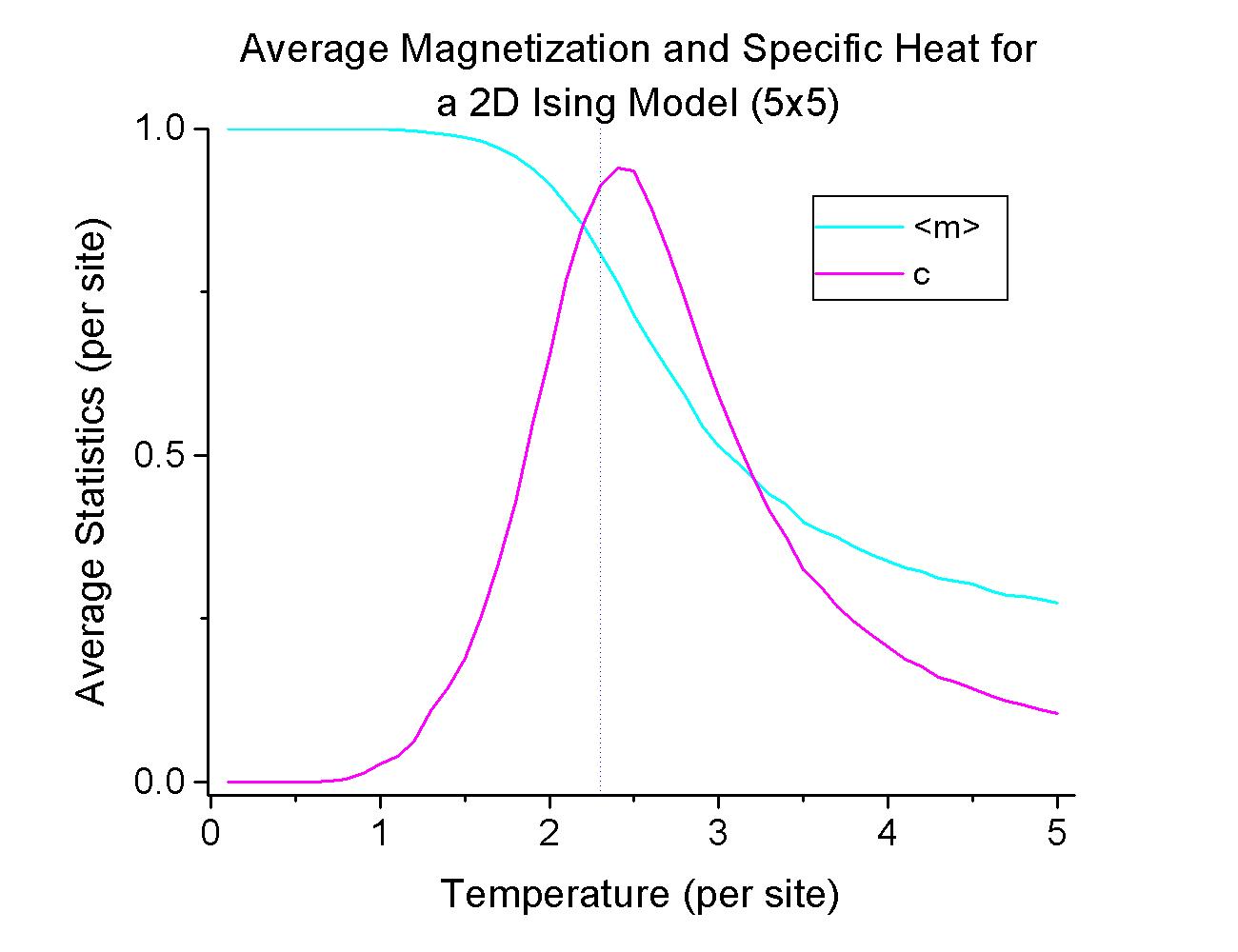
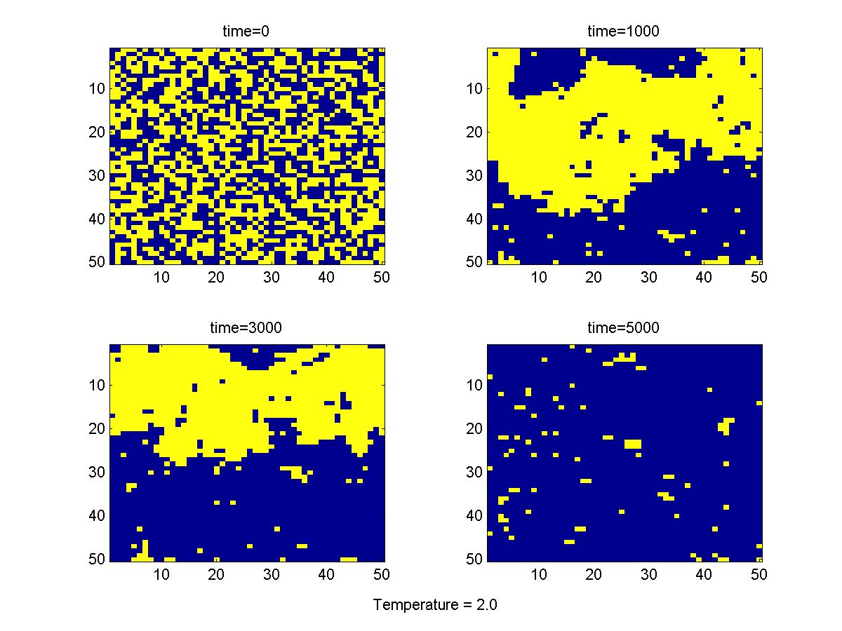
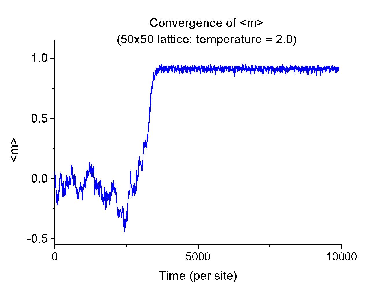
 and c as a function of temperature. You should wait for the system to come to equilibirum (~ 5000 time units) before your calculation of the system's statistics. For good statistical results, you should average your statistical quantities for at least another 5000 time units. Similar to the 5x5 case, you should observe a critical transition near T=2.3.
 and c behave at Tc in the thermodynamic limit (
 )? Disscuss your results.

where X' is the new configuration, X is the old configuration, and siX denotes the spin value at site i in the configuration X.
You should convince yourself the validity of these equations by filling in the intermediate steps.

can only take on a finite discrete set of values. Namely, the sum over all nearest neighbors in the equation for EX'-EX can only take on the following interger values: -z,-z+2,-z+4,...,z where z is the total number of nearest neighbor spins. Instead of calculating the exponential function at every iterations, one should construct a look up table for these values. The program will run much faster with this.
