PHYS 510 - Computational Physics I

Assignment 4: Numerical Integration

Spring 2010

Reading Assignment

1. Chapter 4: Integration of Functions in Press
2. Chapter 5, 6, 7, and 15: Numerical Integration in Landau

Assignment 4

1. Gauss-Hermite Quadrature
   

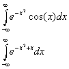
   The Gauss-Hermite Quadratures are suitable for integrals of the following form:
   
   and the quadrature is given by
   
   where x_k are the Guass points and w_k are the weights. Similar to the example done in class, one can calculate these weights and Gauss points by requiring the quadrature to be exact for the following basic monomials functions: {1,x,x²,x³,...}.
   
   

   1. Derive the Guass points and weights for the N=2 order quadrature. Verify that the Guass points in this case correspond to the roots of the Hermite polynomial of order N=2: H₂(r)=4r²-2.
   2. The fifth order Guass points and weights are given below:
      

      Order N	(+ -)xk	wk
      5	0.00000000	0.94530872
      	0.95857246	0.39361932
      	2.02018287	0.01995324

      Calculate the following integrals
      
      using the 2nd and 5th order Gauss-Hermite Quadratures. To within single precision, the 5th order result can be considered as the exact values for the integrals. How accurate is the 2nd order result?

   Solution: hergau.pdf (80k)

   ---

2. Electrostatics
   
   

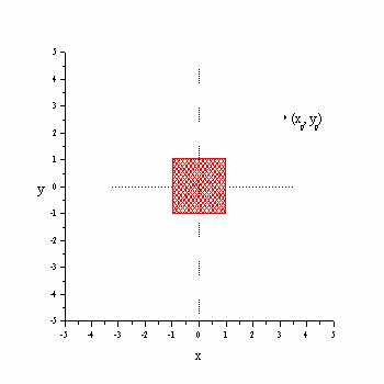
   An uniform charge distribution r is as shown above. It occupies a squre region [-1,1]x[-1,1] in the plane. The electrostatic potential at an observation point (x_p, y_p) due to this charge distribution is obtained by the following integral:
   
   For simplicity, assume r/4pe₀ = 1
   

   1. Write a code to integrate the above equation using the Monte Carlo method.
   2. Write another code to do the same using the Simpson's rule.
   3. Compare the efficiency of the two methods up to single precision accuracy for a randomly chosen observation point (x_p, y_p).
   4. Plot the electrostatic potential everywhere [-5,5]x[-5,5] with at least 4 significant digits accuracy.
   5. Discuss your results

   Solution
   

   An ANSI C implementation of the two algorithms used to integrate the charge density is listed here. A sample output for a random observation point outside the charge distribution is given here:
   For the accuracy of 0.0001, the electric potential is:
   Observation point: [1.5708,1.0472]
   

   • Monte Carlo method: 2.25759 with 10485760 evaluation pts
   • Simpson's Rule: 2.25806 with 385 evaluation pts

   One should note that for roughly 4 significant figures, MC needs orders of magnitude more function evaluations to get close to the result obtained by the Simpson's Rule in this example. [As a side note, one can see that the performance for both methods gets worse if the observation point is inside the charge distribution so that the integrant has large variations near the observation point. In this case, both MC and SR require a large number of function evaluations than previously and SR has a slight advantage in both accuracy and efficiency.]

   The convergence of the Monte Carlo method in dimensions less than 4D as we have seen is slower than the Simpson's rule. The expected rate of convergence for Monte Carlo is 1/sqrt(N), where N is the number of data points used in the estimate. On the other hand, Simpson's rule typically should converge as h⁴. However, as we have disscued in class, the number of points N needed for the Simpson's rule depends on the dimension of the integral. In particular, the number of grid points needed typically scales as N~h^-d, where h is the required grid size. While in 2D, the required N for a given accuracy is still much smaller for the Simpson's rule, N can easily grow to unmanageable size for large d>4D. The advantage of Monte Carlo method is that the number of evaluation points needed is not depended on dimension. Thus, while the convergence of the accuracy of Monte Carlo integral is slow, it might be the ONLY method which will give a rough estimate in these high dimenional integrals. The following is a plot showing the convergence of the 2D MC integrator for the case with [xp,yp]=[1.5708,1.0472] shown above:
   

   A simpler example showing the convergence rate for a 1D MC integral of x² is given below. As you can see in this 1D case, the number of function evaluations is still large for this relatively simple integral and SR can get an accurate answer in just 20 steps.
   

   A modification of the Simpson's Rule from above is used to plot the electric potential as a function of position. The code for this is here and the following is the plot of F(x_p,y_p) as a function of position