SolutionStochastic Differential Equations (SDEs) play a very important role in modeling complex and stochastic systems in fields including statistical physics, biology, and finance. The Fokker-Plank equation in statistical physics and the Black-Scholes equation in modern finance are examples of SDEs and SDEs are indispensable in the analysis of diffusion processes, Brownian motion, population dynamics, and stock prices. Although the theory behind this branch of mathematics is beyond the scoop of this course, the numerical methods used in simulating these systems can be easily learned. (For those interested in learning more about SDEs, check out Math 674 offered by the Department of Mathematical Sciences.)
For this assignment, you need to do the following:
- Read and gain a basic understanding of the article "An Algorithmic Introduction to Numerical Simulation of Stochastic Differential Equations."
- Write a code which can generate a standard Brownian path. This will be the basic subroutine needed for all remaining parts of this problem.
A standard Brownian path will have the following statistical properties: the mean value of W(t), m(W(t))=E[W(t)] should be zero and the variance of W(t), γ(W(t))=E[(W(t)-E[W(t)])2], should be t. Note: E[] is called the expectation value. For numerical applications, E[] can be evaluated as the regular sampled average, i.e.
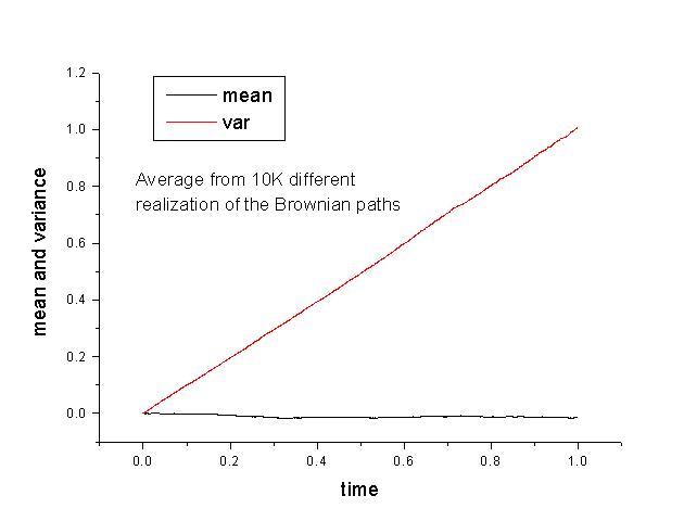
Verify this fact by evaluating m(W(t)) and γ(W(t)) as a function of t from 0 to 1 from an ensemble of 10K different realizations of the Brownian paths.- Many different stochastic processes can be written as functions of the Brownian path. A particular interesting example is called a Brownian bridge which has the characteristic that it is basically a random walk but its starting and ending points are fixed. An example of a Brownian bridge with X(0)=X(1)=0 is given by X(t)=W(t)-tW(1). Use the basic Brownian Path subroutine in part a to generate five different realizations of this Brownian bridge.
- Solution of Linear SDEs: Brownian paths in continuous time is a curious mathematical object. As you can see from the previous two parts, Brownian paths are highly irregular curves. In fact, they are examples of curves which are continuous but nowhere differentiable. Therefore, it doesn't make sense to write dW(t)/dt since W(t) is not a differentiable process. However, one can define integrals of stochastic processes (see Sec. 4 in handout) and stochastic differential equations can be defined in terms of these stochastic integrals. In standard notations, a SDE for a particular stochastic process X(t) can be written in differential forms:
A simple numerical method to integrate this SDE is the Euler-Maruyama method,
where Δt=T/L for some positive integer L, and τj=jΔt. (For more details, see Sec. 4 in handout.)
For a linear SDE, f(X) and g(X) are linear functions of X(t). In particular, we are interested in linear SDE in the form,
This is basically a diffusive process with a linear drift. It is the basic model for stock prices in the well-known Black-Scholes equation. The analytic solution to this linear SDE is given by,
.
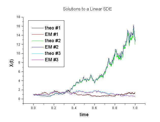
- Implement the Euler-Maruyama algorithm to solve this linear SDE with λ=2, μ=1, and X0=1. Plot a few realizations of X(t) from t=0 to t=1. Compare your results with the theoretical expectation given by Eq. (1).
- The expectation value of X(t), E(X(t)), is given by exp(2t). Verify this by evaluating the average of X(t) from an ensemble of 10K different realizations of X(t).
- Reading
One of the basic assumption for a Brownian process is that for a given time interval dt, the increment of the Brownian process, dW(t)=W(t+dt)-W(t), is a gaussian random variable with mean zero and variance dt. It is also assumed that the increments dW at different time are independent. In other words, dW(t) is a gaussian random variable given by sqrt(dt)N(1,0), where N(1,0) are independent gaussian random numbers given by the normal probability distriuction:
To generate the set of gaussian random number N(1,0), one can use the transformation method given in Press. Since W(t) is a random process, differnt realizations of W(t) will be different. However, as stated above, its mean and variance are well defined. In particular, m(W(t))=0 and γ(W(t))=t. Using 10,000 different realizations of the Brownian paths, this fact is illustrated in the following calculated curve for m(W(t)) and γ(W(t)):

Five realizations of the Brownian bridge: X(t)=W(t)-tW(1), 0<=t<=1, is given below:

Notice that different realizations of a stocastic process can vary significantly. However, for this process, the end points will always be fixed at zero.
The C code which generates these graphs is given here.
We ploted three different realizations of X(t) by solving the linear SDE using the Euler-Maruyama method. Superimposed on top are the analytical solutions of X(t) using Eq. 4.6 (handout). As one can see, they agree quite well. This is the consequence of the fact that the Euler-Maruyama method has a strong order of convergence equal to 1/2. This can be improved to order 1. However, higher order methods such as the RK4 method for deterministic systems do not exist yet. This is still an open area of research.

The expectation value of X(t), E(X(t)), can be calculated exactly to be exp(2t) for this linear stochastic process. In the following graph, we have superimposed this theoretical expectation on top of the numerically calculated E[X(t)] and three sample realizations of X(t). The point is that although each realization of X(t) can vary greatly, the expectation value of X(t) is a well defined quantity in terms of drift λ and spread μ.

The C code which generates these graphs is given here.


