SolutionCoupled oscillators are ubiquitous in nature. A number of physical, chemical, and biological systems can be thought of as a large ensemble of weakly interacting nonidentical oscillators. Examples include pacemaker cells in the heart and brain, synchronously flashing fireflys, coupled laser arrays, and arrays of Josephson junction arrays. One interesting phenomenon common to all these systems is their ability to collectively synchronize, in which a large number of the oscillators lock onto a common frequence despite the difference in their natural frequencies. The simplest of this phenomenon was studied by Kuramoto in 1984 (see reviews by SH Strogatz, Physicsa D, 143 1-20 (2000) and SH Strogatz and I Stewart, Sci. Am, 269 (6) 102 (1993)) for a large population of N weakly coupled periodic oscillators,
where i=1,2,...,N, θi(t) is the phase of the oscillator i, ωi is the natural frequency of the uncoupled oscillator i, and K is the strength of the coupling between oscillators. The phase variable θi is periodic from 0 to 2π. Notice that the sum in the above equation is running over all the oscillators so that this is an example of a globally coupled system.Kuramoto studied this system in term of a complex mean field variable
where r(t) and ψ(t) are the magnitude and phase of this global mean field. Because of the following identity
we can rewrite the Kuramoto model Eq. (1) in terms of the mean field variable r and ψ,
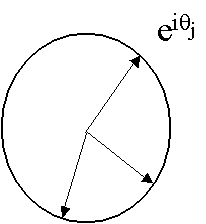
For N large, the globally coupled system will change from a "phase incoherent" state where the individual phase variable θi are not correlated, to a "phase coherent" state where most of the oscillators will tend to clump around the mean phase ψ(t). The transition occurs at a critical coupling strength K* which can be calculated in certain cases. In terms of the mean field variables, the phase incoherent state is characterized by a random distribution of individual phases (see below) and the averge of eiθj over all oscillators (the sum on the right hand side of Eq. (2)) is expected to be close to zero (~N-1/2).
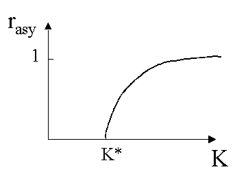
In other words, as N approaches infinity, the magnitude r(t) of the complex mean field after a long time should be zero in the incoherent state with K < K* and r(t) should approach a nonzero asymptotic value rasy in the coherent state with K > K*. Actually, as K increases pass K*, more and more oscillators will be recruited toward the mean phase ψ(t) and rasy is expected to continuously increase from zero to one.

This phase transition for globally coupled periodic oscillators can be studied both analytically and numerically. For this assignment, you need to verify the following theoretical expectations by doing a numerical experiments with the Kuramoto model. You need to solve the N coupled ODEs given by Eq. (3) simultaneously using a RK4 solver with or without adaptative steps. (Note that the coupling in this set of equations is through the mean field variables r(t) and ψ(t).) Since the fluctuations is expected to scale as N-1/2, you should use at least 10000 oscillators for good results. For this experiment, we will pick a Lorentzian distributionn for the natural frequencies of the oscillators,
where ω0 is the mean frequency of the distribution and Δ is the width of the Lorentzian. (Take ω0 = 2 and Δ = 1 for this experiment.)
- Estimate the critical coupling strenght K* by evaluating the asymptotic value rasy as a function of K. [Note: Since the system is of finite size, one can numerically minimize the statistical fluctuations in rasy by averaging it over a duration of time after the asymptotic transience has been taken out.]
- For a Lorentzian distribution of natural frequencies, the expected value of K* is 2Δ. Using your numerical answer from part a) to verify this fact.
- The shape of the function for rasy(K) with K > K* should be a square root dependence,
.
Vertify this fact by plotting rasy vs. (K-K*). For K sufficiently close to K*, this function will have a universal scaling behavior given by
.
If one plots ln rasy vs. ln (K-K*) near the transition point K*, the resulting slope should give 1/2.
To simulate the Lorentzian random numbers, we can use the transformation method discussed in class (also see Press). The transformation needed to convert a uniform distribution of random number to a one distributed according to Eq. 4 is simply the tan function,
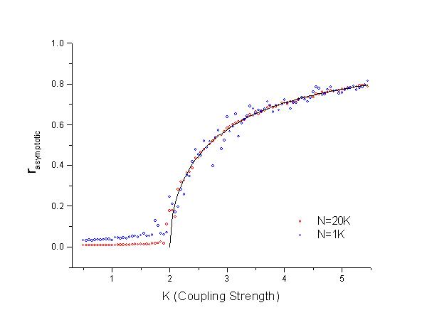
where x is distributed uniformly in [0,1]. The ODE solver used for this problem is the standard RK4 with a step size of 0.1. Since the mean field is an average of N complex numbers, its fluctuations are expect to be in the order of N-1/2. This can be seen in the two different runs on rasy vs. K for two different values of N [N=1000 (blue) and N=20000 (red)].
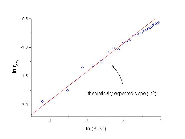
With N=1000, the fluctuations in our curve are roughly on the order of 0.03 and with N=20K, the fluctuations are smaller ~ 0.007. Using the curve with less fluctuations, the critical coupling value K* can be seen to agree with the theoretical expectation of K*=2Δ=2.In order to check the scaling of rasy with K near the critical value K*, we plotted ln rasy vs. ln (K-K*). To further minimize the fluctuations near K*, we rerun our system with N increasing to 50K. The following is the resulting graph.
We have used the theoretical expected value of K*=2 for this graph. As one can see from this graph, for K close K*=2, the scaling is as expected with an exponent of 1/2. As K moves away from the scaling region, there is a crossover to nonuniversal behavior and the exponent deviates from 1/2. In the special case with Lorentzian distributed natural frequencies, the exact solution for rasy is
To leading orders of t=K-K*, the above expression can be written as
The exact solution Eq. 5 for a network of Lorentzian distributed oscillators is plotted as a thin black line in the first figure.The C implementation of this problem is given here.


