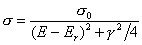
The cross section for a resonant scattering experiment of a neutron from a nucleus is given by the following table:
E(Mev) 0 25 50 75 100 125 150 175 200 sexp(mb) 10.6 16.0 45.0 83.5 52.8 19.9 10.8 8.25 4.7 For data analysis and presentation, you are asked to determine values for the cross section at energies between the measured values. In general, there are two different approaches to this problem.
- Numerically interpolate the values of sexp given in the table. This will be useful, if a priorly, we don't have a mathematical expression for our theoretical expectation. On the other hand, since interpolation will find a function going through ALL data points, it might provide spurious results if the data are contaminated by experimental noise.
- Numerically best fit the data to a pre-determined function. By the construction of the least-square fit algorithm (which we will discuss in a later chapter), effects of experimental noise will be statistically minimized in the resulting best fitted function. However, we need to come up with a physically resonable mathematical model for the data first.
In this exercise, we assume that we don't have a theoretical model for this process and we simply want to interpolate the measured data. Please complete the following tasks:
This is a demonstration showing that higher order interpolation does not necessary imply higher accuracy.
- Use the improved Neville's algorithm to fit the entire experimental spectrum with one polynomial. This means using an eight degree polynomial to interpolated the nine data points. Use the interpolated values to plot the cross section in steps of 5 Mev.
- A more reasonable use of interpolation algorithms is to model LOCAL behvaior with a small number of data points. Redo the interpolation of the cross section data with only three data points at a time. Plot the resulting piece-wise continuous interpolating polynomials in 5 Mev steps.
- The actual theoretical model for this scattering process is given by the Breit-Wigner function:
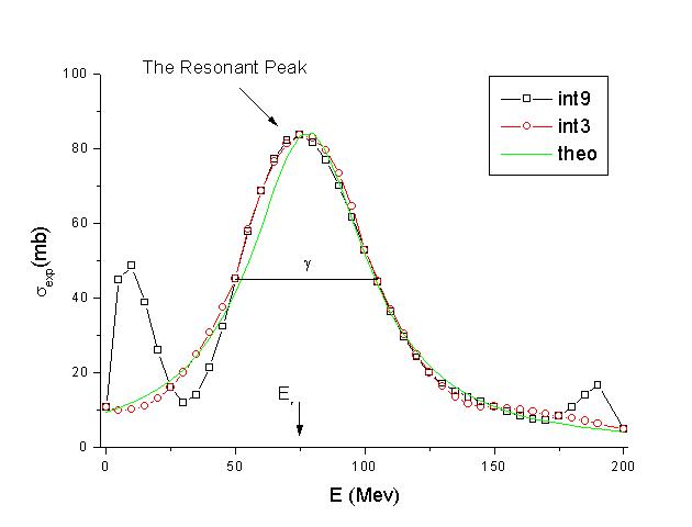
where Er is the resonant energy and g is the full width at half maximum of this resonant process. Using your three-points interpolation algorithm, what is deduced values for Er (the location of the resonant peak) and g (its full width at half max) from your data. Compare these values with the following theoretical values: s0=6.389x10⁴, Er=78, and g= 55 for this particular data set. Plot the theoretical prediction on top of the two interpolated curves.
Solutions
You can find a C implementation of this problem's solution in resonante.c. This program performs the 9 points improved Neville's algorithm, the 3 points improved Neville's algorithm, and plots the theortical resonant curve. The output resonante.dat is a tab delimited text file with four columns: E, int9, int3, and theo. The interpolated and theoretical curves are plotted with a resolution of 5 Mev. The following is a graph of these curves.
Using the 3 points interpolation and with a resolution of 5 Mev, Er is estimated to be at 75 Mev and the full width at half max g is estimated to be 55. Although both the 9 points and 3 points interpolations give good estimate of the location and the width of the central peak, the higher order interpolation with 9 data points generates more spurious oscillations in the estimated resonant curve. These spurious peaks are especially obviously at the low and high energy ranges. On the other hand, the 3 points interpolation approximates the theoretical curve closely. One drawback is that the 3 points interpolated curve is only piece-wise differentiable. The derivative discontineously changes every two data intervals.
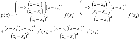
Hermite Interpolation Equation click
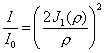
Airy Pattern describes the intensity profile of the diffraction pattern from a circular aperture. Using the two points Hermite interpolation, write a program to evaluate the relative intensity I/I0 = (2J1(r)/r)2 as a function of r across the Airy Pattern from r=0 to r=10, and plot it. To generate a "pleasing" display, you should evaluate the intensity at 0.1 increments in r. In conjunction with a root-finder (choose anyone from last chapter), determine the r- value for which the intensity is zero, i.e., find the location of the first fringe in the diffraction pattern.Use the following values for your interpolations:
r J0(r) J1(r) J2(r) 0.0 1.0 0.0 0.0 1.0 0.7651976866 0.4400505857 0.1149034849 2.0 0.2238907791 0.5767248078 0.3528340286 3.0 -0.2600519549 0.3390589585 0.4860912606 4.0 -0.3971498099 -0.0660433280 0.3641281459 5.0 -0.1775967713 -0.3275791376 0.0465651163 6.0 0.1506452573 -0.2766838581 -0.2428732100 7.0 0.3000792705 -0.0046828235 -0.3014172201 8.0 0.1716508071 0.2346363469 -0.1129917204 9.0 -0.0903336112 0.2453117866 0.1448473415 10.0 -0.2459357645 0.0434727462 0.2546303137
Solution
With a knowledge of the function as well as its derivative at tabulated data points, one can use higher order interpolation with less points. The Hermite interpolation algorithm used here uses a cubic interpolation with two data points. An additional advantage of this interpolation method is that both the function and its derivative are continuous across the data intervals. A C implementation of the solution of this problem is airy.c. There are two options for this program. The first choice will plot the Airy pattern at 0.1 increments from r=0 to 10. The other choice willl use the Bisection method to find the location of the first fringe. The relative intensity is positive for all values of r and the zeros of this function are also the local minimums. A numerical search of zeros using the actual relative intensity equation will be difficult. A much simplier algorithm is to look for zeros of the numerator which is simply the Bessel function. The first fringe is found to be at r = 3.8318042146766.
